griddata

mipylib.numeric.minum.griddata(points, values, xi=None, **kwargs)

Interpolate scattered data to grid data.

Parameters

• points – (list) The list contains x and y coordinate arrays of the scattered data.

• values – (array_like) The scattered data array.

• xi – (list) The list contains x and y coordinate arrays of the grid data. Default is None, the grid x and y coordinate size were both 500.

• method – (string) The interpolation method. [idw | cressman | neareast | inside | inside_min | inside_max | inside_count | surface]

• fill_value – (float) Fill value, Default is nan.

• pointnum – (int) Only used for ‘idw’ method. The number of the points to be used for each grid value interpolation.

• radius – (float) Used for ‘idw’, ‘cressman’ and ‘neareast’ methods. The searching raduis. Default is None in ‘idw’ method, means no raduis was used. Default is [10, 7, 4, 2, 1] in cressman method.

• convexhull – (boolean) If the convexhull will be used to mask result grid data. Default is False.

Returns

(array) Interpolated grid data (2-D array)

Examples

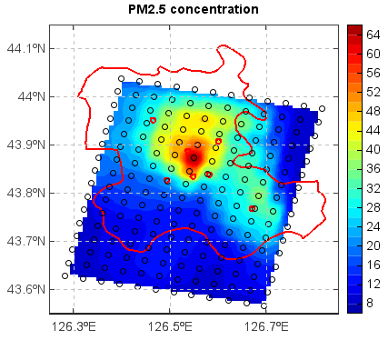
f = addfile('D:/temp/nc/out.20140421_20140421_JL3KMmeic.nc')
data = f['PM25']
data = data[15,1,:,:]
lon = f['lon'][:,:]
lat = f['lat'][:,:]
#Interpolate data to grid
lon1 = linspace(lon.min(), lon.max(), lon.dimlen(1)*5)
lat1 = linspace(lat.min(), lat.max(), lat.dimlen(0)*5)
data1 = griddata((lon, lat), data, xi=(lon1, lat1), method='idw', convexhull=True)[0]
lon_g,lat_g = meshgrid(lon1, lat1)
#Plot
axesm()
mlayer = shaperead('D:/temp/map/jilin.shp')
geoshow(mlayer, edgecolor='r', size=2)
layer = contourfm(lon1, lat1, data1, 20)
scatterm(lon, lat, data, 20, fill=False)
colorbar(layer)
xlim(126.25,126.85)
ylim(43.55,44.15)
grid(True)
title('PM2.5 concentration')