particles
- Axes3DGL.particles(*args, **kwargs):
creates a three-dimensional particles plot
- Parameters:
x – (array_like) Optional. X coordinate array.
y – (array_like) Optional. Y coordinate array.
z – (array_like) Optional. Z coordinate array.
data – (array_like) 3D data array.
s – (float) Point size.
cmap – (string) Color map string.
vmin – (float) Minimum value for particle plotting.
vmax – (float) Maximum value for particle plotting.
alpha_min – (float) Minimum alpha value.
alpha_max – (float) Maximum alpha value.
density – (int) Particle density value.
- Returns:
Legend
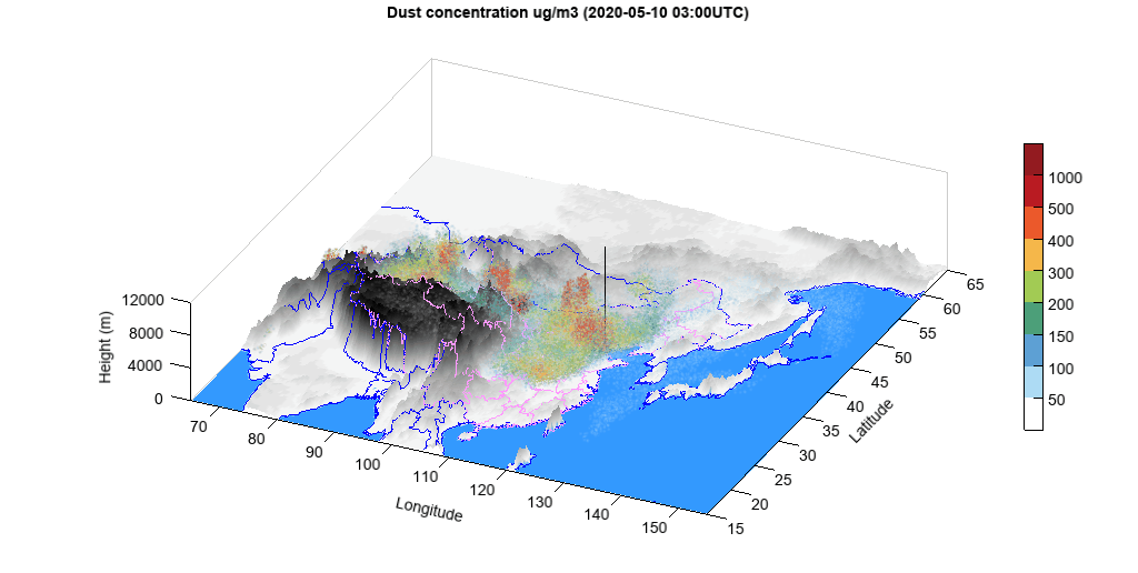
Example of plotting 3d dust concentrations from dust model
#Set date
sdate = datetime.datetime(2020, 5, 11, 0)

#Set directory
datadir = r'W:\Asia-dust\CMA'
datadir = os.path.join(datadir, sdate.strftime('%Y%m%d'))

#Read data
fn = os.path.join(datadir, 'CUACE-DUST_CMA_{}.nc'.format(sdate.strftime('%Y%m%d%H')))
f = addfile(fn)
st = f.gettime(0)
t = 4
dust = f['CONC_DUST'][t]
levels = dust.dimvalue(0)
#dust[dust<5] = 0
height = meteolib.pressure_to_height_std(levels)
lat = dust.dimvalue(1)
lon = dust.dimvalue(2)

#Relief data
rfn = 'D:/Temp/nc/elev.0.25-deg.nc'
rf = addfile(rfn)
elev = rf['data'][0,'15:65','65:155']
elev[elev<0] = -1
lon1 = elev.dimvalue(1)
lat1 = elev.dimvalue(0)
lon1, lat1 = meshgrid(lon1, lat1)

#Map
lchina = shaperead('cn_province')
clon = lchina.x_coord
clat = lchina.y_coord
calt = zeros(len(clon))
h = interp2d(elev, clon, clat)
calt = calt + h
lworld = shaperead('country')
wlon = lworld.x_coord
wlat = lworld.y_coord
walt = zeros(len(wlon))
h = interp2d(elev, wlon, wlat)
walt = walt + h

#Plot
ax = axes3d()
ax.set_elevation(-20)
ax.set_rotation(335)
rlevs = arange(0, 6000, 200)
cols = makecolors(len(rlevs) + 1, cmap='MPL_gist_yarg', alpha=1)
cols[0] = [51,153,255]
surf(lon1, lat1, elev, rlevs, facecolor='interp', colors=cols, edge=False)
plot3(clon, clat, calt, color=[255,153,255])
plot3(wlon, wlat, walt, color='b')
#Beijing location
plot3([116.39,116.39], [39.91,39.91], [0,12000])
#lighting(position=[1,1,1,1], mat_specular=[0.5,0.5,0.5,1])
levs = [50,100,200,300,400,500]
#levs = [100,200,300,400,500]
cmap='WhiteBlueGreenYellowRed'
#cmap = 'MPL_Oranges'
pp = particles(lon, lat, height, dust, levs, vmin=20, s=2, \
    cmap=cmap, alpha_min=0.1, alpha_max=0.7, density=1)
colorbar(pp, aspect=30)
xlim(65, 155)
xlabel('Longitude')
ylim(15, 65)
ylabel('Latitude')
zlim(0, 12000)
zlabel('Height (m)')
tt = st + datetime.timedelta(hours=t*3)
title('Dust concentration ug/m3 ({}UTC)'.format(tt.strftime('%Y-%m-%d %H:00')))
#savefig('D:/Temp/test/dust_3d_{}.png'.format(tt.strftime('%Y%m%d%H')), dpi=150)
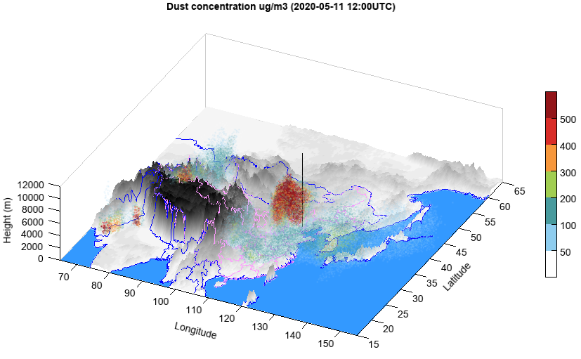
Example of output gif animation of 3d dust concentrations from dust model
import time

#Set date
sdate = datetime.datetime(2020, 5, 10, 0)

#Set directory
datadir = r'W:\Asia-dust\CMA'
datadir = os.path.join(datadir, sdate.strftime('%Y%m%d'))

#Read data
fn = os.path.join(datadir, 'CUACE-DUST_CMA_{}.nc'.format(sdate.strftime('%Y%m%d%H')))
f = addfile(fn)
st = f.gettime(0)
t = 0
dust = f['CONC_DUST'][t]
levels = dust.dimvalue(0)
#dust[dust<5] = 0
height = meteolib.pressure_to_height_std(levels)
lat = dust.dimvalue(1)
lon = dust.dimvalue(2)

#Relief data
rfn = 'D:/Temp/nc/elev.0.25-deg.nc'
rf = addfile(rfn)
elev = rf['data'][0,'15:65','65:155']
elev[elev<0] = -1
lon1 = elev.dimvalue(1)
lat1 = elev.dimvalue(0)
lon1, lat1 = meshgrid(lon1, lat1)

#Map
lchina = shaperead('cn_province')
clon = lchina.x_coord
clat = lchina.y_coord
calt = zeros(len(clon))
h = interp2d(elev, clon, clat)
calt = calt + h
lworld = shaperead('country')
wlon = lworld.x_coord
wlat = lworld.y_coord
walt = zeros(len(wlon))
h = interp2d(elev, wlon, wlat)
walt = walt + h

#Plot
ax = axes3d()
ax.set_elevation(-20)
ax.set_rotation(335)
rlevs = arange(0, 6000, 200)
cols = makecolors(len(rlevs) + 1, cmap='MPL_gist_yarg', alpha=1)
cols[0] = [51,153,255]
surf(lon1, lat1, elev, rlevs, facecolor='interp', colors=cols, edge=False)
plot3(clon, clat, calt, color=[255,153,255])
plot3(wlon, wlat, walt, color='b')
#Beijing location
plot3([116.39,116.39], [39.91,39.91], [0,12000])
#lighting(position=[1,1,1,1], mat_specular=[0.5,0.5,0.5,1])
levs = [50,100,150,200,300,400,500,1000]
cmap='WhiteBlueGreenYellowRed'
#cmap = 'MPL_Oranges'

#Loop
giffn = os.path.join(datadir, 'Dust_3d_particles_relief_{}--loop-1.gif'.format(st.strftime('%Y%m%d')))
print giffn
animation = gifanimation(giffn)
tn = f.timenum()
tn = 24
for t in range(1, tn):
    print t
    if t > 1:
        cll()
    dust = f['CONC_DUST'][t]
    pp = particles(lon, lat, height, dust, levs, vmin=20, s=2, \
        cmap=cmap, alpha_min=0.1, alpha_max=0.7, density=1)
    colorbar(pp, newlegend=False, aspect=30)
    xlim(65, 155)
    xlabel('Longitude')
    ylim(15, 65)
    ylabel('Latitude')
    zlim(0, 12000)
    zlabel('Height (m)')
    #zticks(arange(len(levels))[1:], levels[1:])
    tt = f.gettime(t)
    title('Dust concentration ug/m3 ({}UTC)'.format(tt.strftime('%Y-%m-%d %H:00')))
    #Add frame to gif animation
    gifaddframe(animation, width=1024, height=516)

#Finish gif animation
animation.finish()
print 'Finished...'