plot_isosurface

Axes3DGL.plot_isosurface(*args, **kwargs):

creates a three-dimensional isosurface plot

Parameters

• x – (array_like) Optional. X coordinate array.

• y – (array_like) Optional. Y coordinate array.

• z – (array_like) Optional. Z coordinate array.

• data – (array_like) 3D data array.

• cmap – (string) Color map string.

• nthread – (int) Thread number.

Returns

Legend

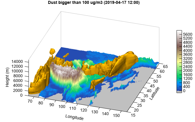
Example of plotting 3d isosurface of dust concentrations from dust model

#Set date
sdate = datetime.datetime(2019, 4, 17, 0)

#Set directory
datadir = 'D:/Temp/mm5'

#Read data
fn = os.path.join(datadir, 'WMO_SDS-WAS_Asian_Center_Model_Forecasting_CUACE-DUST_CMA_'+ sdate.strftime('%Y%m%d%H') + '.nc')
f = addfile(fn)
st = f.gettime(0)
t = 10
dust = f['CONC_DUST'][t,:,:,:]
levels = dust.dimvalue(0)
dust[dust<5] = 0
height = meteolib.pressure_to_height_std(levels)
lat = dust.dimvalue(1)
lon = dust.dimvalue(2)

#Relief data
fn = 'D:/Temp/nc/elev.0.25-deg.nc'
f = addfile(fn)
elev = f['data'][0,'15:65','65:155']
elev[elev<0] = -1
lon1 = elev.dimvalue(1)
lat1 = elev.dimvalue(0)
lon1, lat1 = meshgrid(lon1, lat1)

#Plot
ax = axes3dgl(bbox=True)
ax.set_rotation(348)
ax.set_elevation(-29)
ax.set_lighting(True)
levs = arange(0, 6000, 200)
cols = makecolors(len(levs) + 1, cmap='MPL_terrain')
cols[0] = 'w'
ls = ax.plot_surface(lon1, lat1, elev, levs, colors=cols, edge=False)
ax.plot_isosurface(lon, lat, height, dust, 100, color=[255,180,0,10], \
    edge=False, nthread=4)
colorbar(ls)
xlim(65, 155)
xlabel('Longitude')
ylim(15, 65)
ylabel('Latitude')
zlim(0, 15000)
zlabel('Height (m)')
#zticks(arange(len(levels))[1:], levels[1:])
tt = st + datetime.timedelta(hours=t*3)
title('Dust bigger than 100 ug/m3 (%s)' % tt.strftime('%Y-%m-%d %H:00'))