3-D plots without OpenGL

Create a 3D axes without OpenGL using ax = axes3d(opengl=False), then use the plot functions of the 3D axes object (ax) to plot 3D plots. The functions includes: including plot(), scatter(), contour(), contourf(), imshow(), plot_surface(), plot_wireframe() and plot_layer.

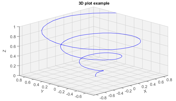
Line plots:

z = linspace(0, 1, 100)
x = z * np.sin(20 * z)
y = z * np.cos(20 * z)

#Plot
ax = axes3d(opengl=False)
ax.plot(x, y, z, '-b')
title('3D plot example')

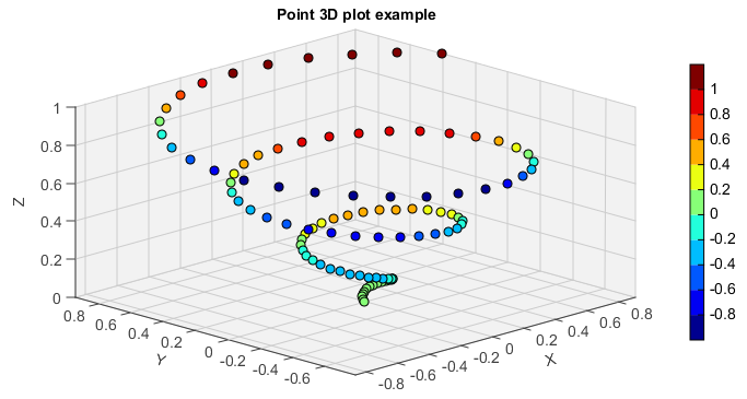
Scatter plots:

z = linspace(0, 1, 100)
x = z * np.sin(20 * z)
y = z * np.cos(20 * z)
c = x + y

#Plot
ax = axes3d(opengl=False)
points = ax.scatter(x, y, z, c=c)
colorbar(points,shrink=0.8)
title('Point 3D plot example')

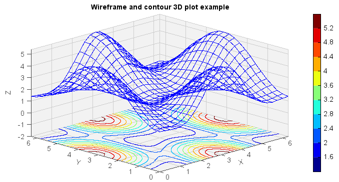
Wireframe and contour plots:

alpha = 0.7
phi_ext = 2 * pi * 0.5
N = 25
x1 = linspace(0, 2*pi, N)
y1 = linspace(0, 2*pi, N)
x,y = meshgrid(x1, y1)
z = 2 + alpha - 2 * cos(y) * cos(x) - alpha * cos(phi_ext - 2 * y)
z = z.T

#Plot
ax = axes3d(opengl=False)
lines = ax.contour(x1, y1, z, 10, offset=-2)
ax.plot_wireframe(x, y, z, color='b')
colorbar(lines)
title('Wireframe and contour 3D plot example')

Wireframe and contourf plots:

alpha = 0.7
phi_ext = 2 * pi * 0.5
N = 25
x1 = linspace(0, 2*pi, N)
y1 = linspace(0, 2*pi, N)
x,y = meshgrid(x1, y1)
z = 2 + alpha - 2 * cos(y) * cos(x) - alpha * cos(phi_ext - 2 * y)
z = z.T

#Plot
ax = axes3d(opengl=False)
lines = ax.contourf(x1, y1, z, 10, offset=-2)
ax.plot_wireframe(x, y, z, color='b')
colorbar(lines)
title('Wireframe and contourf 3D plot example')

Surface plots:

alpha = 0.7
phi_ext = 2 * pi * 0.5
x = linspace(0, 2*pi, 100)
y = linspace(0, 2*pi, 100)
x,y = meshgrid(x, y)
z = 2 + alpha - 2 * cos(y) * cos(x) - alpha * cos(phi_ext - 2 * y)
z = z.T

#Plot
ax = axes3d(opengl=False)
ls = ax.plot_surface(x, y, z, 20, edge=False)
colorbar(ls,shrink=0.8)
title('Surface 3D plot example')

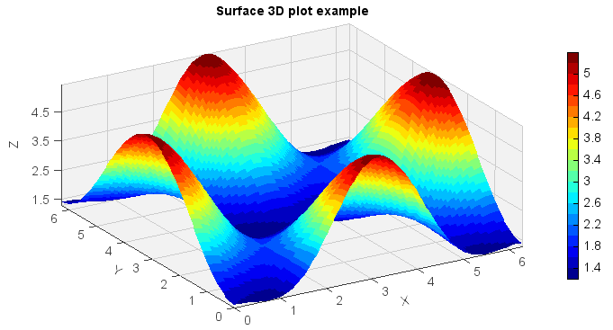
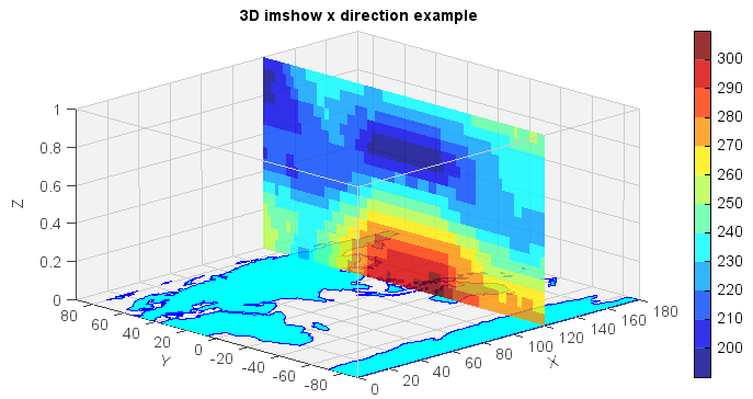
Image plots:

fn = 'D:/Temp/nc/air_clm.nc'
f = addfile(fn)
ps = f['aveair'][0,:,:,'120']
yy = linspace(0, 1., ps.shape[0])
ps.setdimvalue(0, yy)

#Map layer
layer = shaperead('D:/Temp/map/110m-land.shp')

#Plot
ax = axes3d(opengl=False)
ax.plot_layer(layer, color='c', edgecolor='b')
ls = ax.imshow(ps, 10, offset=120, zdir='x', alpha=0.8)
colorbar(ls)
zlim(0, 1)
xlim(0, 180)
title('3D imshow x direction example')

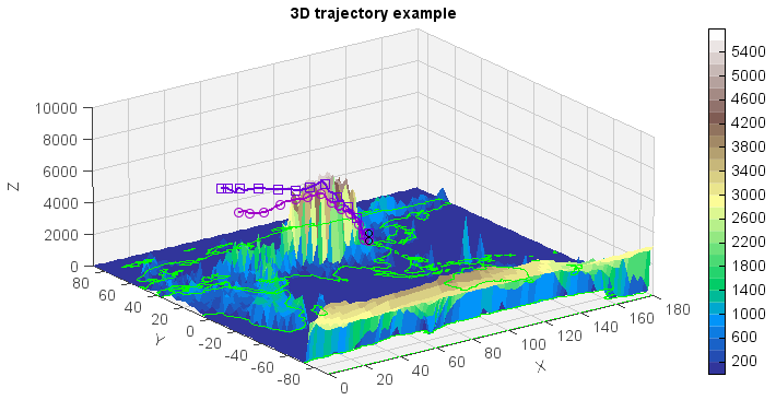
Trajectory plots:

#Open trajectory data and get trajectory layer
fn = 'D:/Temp/HYSPLIT/traj_20131211_00'
f = addfile_hytraj(fn)
lon = f['lon'][:]
lat = f['lat'][:]
alt = f['height'][:]
pres = f['PRESSURE'][:]

#Relief data
fn = 'D:/Temp/nc/elev.0.25-deg.nc'
f = addfile(fn)
elev = f['data'][0,::8,::8]
elev = elev[:,'0:180']
elev[elev<0] = 0

#Plot
ax = axes3d(opengl=False)
surf(elev, 20, cmap='MPL_terrain', edge=False)
geoshow('coastline', facecolor='g')
traj = plot3(lon, lat, alt, mvalues=pres, linewidth=2)
scatter3(lon[:,0], lat[:,0], alt[:,0], marker='o', fill=False,
    size=14, edgecolor='gray')
zlim(0, 10000)
xlim(0, 180)
colorbar(traj, shrink=0.8, aspect=30)
title('3D trajectory example')