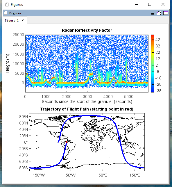
CloudSAT Swath data
Open CloudSAT swath HDF data file and add two plots in a figure. Top one is radar reflectivity factor image on time and height dimensions. Bottom one is satellite trajectory map plot.
# Add file
f = addfile('D:/Temp/hdf/2010128055614_21420_CS_2B-GEOPROF_GRANULE_P_R04_E03.hdf')

# Read data
vname = 'Radar_Reflectivity'
v_data = f[vname]
data = v_data[:,:]
v_height = f['Height']
height = v_height[0,:]
time = f['Profile_time'][:]
lon = f['Longitude'][:]
lat = f['Latitude'][:]

# Read attributes
long_name = v_data.attrvalue('long_name')[0]
scale_factor = v_data.attrvalue('factor')[0]
valid_min = v_data.attrvalue('valid_range')[0]
valid_max = v_data.attrvalue('valid_range')[1]
units = v_data.attrvalue('units')[0]
units_h = v_height.attrvalue('units')[0]

# Apply scale factor
valid_max = valid_max / scale_factor
valid_min = valid_min / scale_factor
data = data / scale_factor
data[data>valid_max] = nan
data[data<valid_min] = nan
data = data.T
data = data[::-1]

# Make a split window plot
subplot(2, 1, 1)

# Contour the data
levs = arange(-38, 50, 2)
layer = imshow(time, height[::-1], data, levs)
colorbar(layer)
title('Radar Reflectivity Factor')
xlabel('Seconds since the start of the granule. (seconds)')
ylabel('Height (m)')

# The 2nd plot is the trajectory
subplot(2, 1, 2)
axesm(newaxes=False)
geoshow('country', edgecolor='k')
plot(lon, lat, '-b', linewidth=4)
#scatter(lon, lat, lon, size=4, edge=False, facecolor='b')
scatter(lon[0], lat[0], size=6, facecolor='r')
xlim(-180, 180)
ylim(-90, 90)
title('Trajectory of Flight Path (starting point in red)')