Himawari-8 data
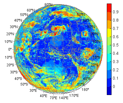
This example code illustrates how to access and visualize a Himawari-8 data (http://www.eorc.jaxa.jp/ptree/index.html). It is very hight resolution data with 22000 and 22000 of x and y dimensions, so the step is set to 4 to reduce the memory usage.
#Add data file
fn = 'D:/Temp/nc/IDE00220.201507140300.nc'
f = addfile(fn)

#Get data variable
v = f['channel_0003_brf']
data = v[0,::4,::4]
data = data[::-1,:]

#Plot
ax = axesm(proj='geos', lon_0=104.7, h=35785863, gridlabel=True, gridline=True, frameon=False)
geoshow('country')
levs = arange(0, 1, 0.1)
layer = imshow(data, levs, proj=ax.proj)
colorbar(layer)
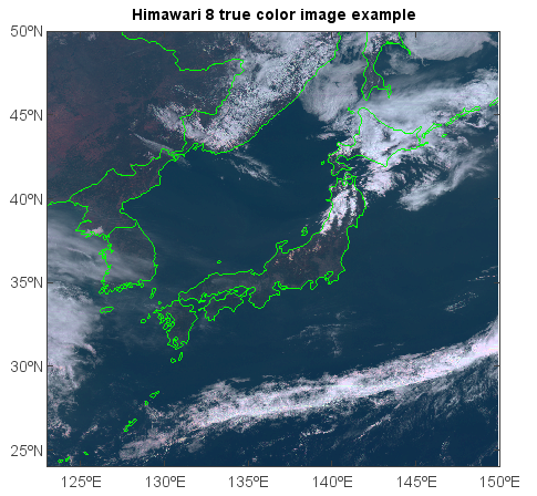
The sample code to create Himawari-8 true color image from band 1 (blue), 2 (green) and 3 (red).
#Add data file
fn = r'C:\Temp\himawari8\NC_H08_20170508_0040_r14_FLDK.02701_02601.nc'
f = addfile(fn)

#Read data
bdata = f['albedo_01'][:,:]
gdata = f['albedo_02'][:,:]
rdata = f['albedo_03'][:,:]
bdata[bdata>1] = 1
gdata[gdata>1] = 1
rdata[rdata>1] = 1

#Plot
axesm()
geoshow('country', edgecolor='g')
layer = imshowm([rdata,gdata,bdata])

#Adjust image
imagelib.hsb_adjust(layer, h=0, s=0.1, b=0.2)
title('Himarari 8 true color image example')
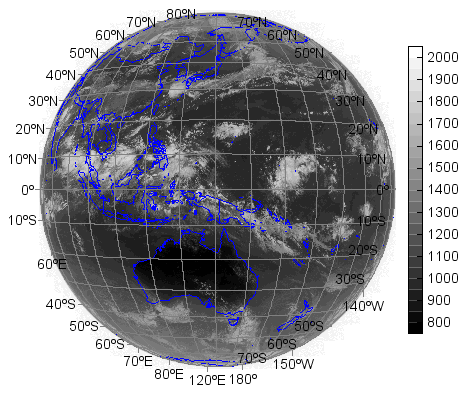
Himawari Standard Data (HSD) format was described in the document http://www.data.jma.go.jp/mscweb/en/himawari89/space_segment/hsd_sample/HS_D_users_guide_en_v12.pdf . The example to read and plot HSD data:
import struct

def read_h8(fn):
    #Read data header
    f = open(fn, 'rb')
    hlen = 0
    #1 Basic information block
    f.read(282)
    hlen += 282
    #2 Data information block
    f.read(5)
    ncol, = struct.unpack('<h', f.read(2))
    nrow, = struct.unpack('<h', f.read(2))
    f.read(41)
    hlen += 50
    #3 Projection information block
    #f.read(127)
    f.read(19)
    sx, = struct.unpack('<f', f.read(4))
    sy, = struct.unpack('<f', f.read(4))
    f.read(127 - 27)
    hlen += 127
    #4 Navigation information block
    f.read(139)
    hlen += 139
    #5 Calibration information block
    f.read(147)
    hlen += 147
    #6 Inter-calibration information block
    f.read(259)
    hlen += 259
    #7 Segment information block
    #f.read(47)
    f.read(3)
    tns, = struct.unpack('b', f.read(1))
    ssn, = struct.unpack('b', f.read(1))
    fln, = struct.unpack('<h', f.read(2))
    f.read(40)
    hlen += 47
    #8 Navigation correction information block
    f.read(1)
    blen, = struct.unpack('<h', f.read(2))
    f.read(blen - 3)
    hlen += blen
    #9 Observation time information block
    f.read(1)
    blen, = struct.unpack('<h', f.read(2))
    f.read(blen - 3)
    hlen += blen
    #10 Error information block
    f.read(1)
    blen, = struct.unpack('<h', f.read(2))
    f.read(blen - 3)
    hlen += blen
    #11 Spare block
    f.read(259)
    hlen += 259

    f.close()

    #Read data
    data = binread(fn, [nrow, ncol], 'short', skip=hlen)
    data = data.astype('float')
    data[data<0] = nan
    return data, ncol, nrow, fln

#Read data files
segments = range(1, 11)
for segment in segments:
    fn = 'E:/Temp/himawari8/HS_H08_20170921_0410_B16_FLDK_R20_S%02i10.DAT' % segment
    print fn
    data1,ncol,nrow1,fln1 = read_h8(fn)
    if segment == segments[0]:
        data = data1
        fln = fln1
        nrow = nrow1
    else:
        data = concatenate([data, data1], axis=0)
        nrow += nrow1
data = data[::-1,:]

#Plot
sx = -5500000
sy = 5500000 - segments[-1] * 550 * 2000
x = arange1(sx, ncol, 2000)
y = arange1(sy, nrow, 2000)
ax = axesm(proj='geos', lon_0=140.7, h=35785863, gridlabel=True, gridline=True, frameon=False)
geoshow('country', edgecolor='b')
cmap = 'MPL_gist_gray'
levs = arange(800, 2001, 50)
layer = imshowm(x, y, data, levs, cmap=cmap, proj=ax.proj)
colorbar(layer, shrink=0.8)