曲线拟合（numeric.fitting）

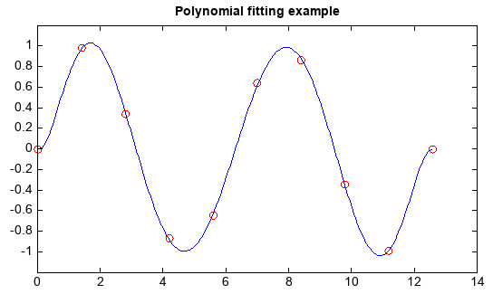
numeric.fitting包中包含了一些曲线拟合函数：expfit – 指数函数拟合；polyfit – 多项式拟合；powerfit – 幂函数拟合。 下面给出一个多项式拟合的例子：

x = linspace(0, 4*pi, 10)
y = sin(x)

#Plot data points
plot(x, y, 'ro', fill=False, size=1)

#Use polyfit to fit a 7th-degree polynomial to the points
r = fitting.polyfit(x, y, 7)

#Plot fitting line
xx = linspace(0, 4*pi, 100)
p = r[0]
yy = fitting.polyval(p, xx)
plot(xx, yy, '-b')
title('Polynomial fitting example')

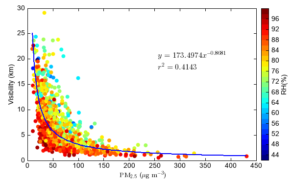
“MeteoInfo -> sample -> ASCII”目录中的pm_vis_rh.txt文件中包含了PM2.5浓度、能见度和相对湿度数据，通常PM2.5 浓度和能见度有较好的幂函数关系，可以用powfit函数进行拟合。

fn = os.path.join(migl.get_sample_folder(), 'ASCII', 'pm_vis_rh.txt')
df = DataFrame.read_table(fn, format='%3f')
pm = df['PM2.5'].values
vis = df['VIS'].values
rh = df['RH'].values

#Plot data scatter points
ls = scatter(pm, vis, s=8, c=rh, cmap='NCV_jet', edgecolor=None, cnum=20)
xlim(0, 450)
ylim(0, 30)
xlabel(r'$\rm{PM_{2.5}} \ (\mu g \ m^{-3})$')
ylabel('Visibility (km)')
colorbar(ls, label='RH(%)')

#Pow law fitting
a, b, r, f = fitting.powerfit(pm, vis, func=True)

#Plot fitting line
xx = linspace(pm.min(), pm.max(), 100)
yy = fitting.predict(f, xx)
plot(xx, yy, '-b', linewidth=2)
text(250, 20, r'$y = ' + '%.4f' % a + 'x^{%.4f' % b + '}$', fontsize=16)
text(250, 18, r'$r^2=%.4f' % r + '$', fontsize=16)