统计分析（numeric.stats）

numeric.stats包中包含了一些统计分析函数：percentile函数用来计算多维数组沿某一特定轴的任意百分比分位数； covariance函数用来计算两个数组的协方差；cov函数用来计算数组的协方差矩阵；

>>> a = array([[10, 7, 4], [3, 2, 1]])
>>> stats.percentile(a, 25)
1.75
>>> stats.percentile(a, 50, axis=0)
array([6.5, 4.5, 2.5])
>>> x1 = [12, 2, 1, 12, 2]
>>> x2 = [1, 4, 7, 1, 0]
>>> stats.covariance(x1, x2)
-7.28
>>> stats.cov(x1, x2)
array([[32.2, -9.1]
      [-9.1, 8.3]])

pearsonr函数用来计算两个数组的皮尔逊相关系数；spearmanr函数用来计算斯皮尔曼相关系数；kendalltau函数用来计算肯德尔 相关系数。

>>> y = [29.81,30.04,41.7,43.71,28.75,37.73,52.25,32.41,25.67,28.17,25.71,36.05,37.62,34.28,38.82,40.15,35.69,28.36,39.56,52.56,54.14,50.76,39.35,43.16,nan]
>>> x = [51.6,46,64.3,83.4,65.9,49.5,88.6,101.4,55.9,41.8,33.4,57.3,66.5,40.5,72.3,70,83.3,65.8,63.1,83.4,102,94,77,77,nan]
>>> stats.pearsonr(x, y)
(0.700798023949337, 0.00013671344970870593)
>>> y = [1,2,3,4,5]
>>> x = [5,6,7,8,7]
>>> stats.spearmanr(x, y)
array([[1.0, 0.8207826816681233]
      [0.8207826816681233, 1.0]])
>>> x1 = [12, 2, 1, 12, 2]
>>> x2 = [1, 4, 7, 1, 0]
>>> stats.kendalltau(x1, x2)
-0.47140452079103173

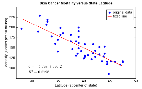
linregress函数用来进行线性回归分析，可以计算出两个数组线性回归的斜率、截距、相关系数、p值、标准差。“MeteoInfo -> sample -> ASCII”目录中的skincancer.txt文件中包含了纬度和皮肤癌死亡率的数据，下面的例子对该数据进行线性回归分析。

fn = os.path.join(migl.get_sample_folder(), 'ASCII', 'skincancer.txt')
df = DataFrame.read_table(fn, format='%s%f%2i%f')
lat = df['Lat'].values
mort = df['Mort'].values

slope, intercept, r, p, std_err = stats.linregress(lat, mort)
scatter(lat, mort, label='original data', edge=False)
plot(lat, intercept+slope*lat, 'r', label='fitted line')
text(29, 100, r'$\hat{y} = ' + '%.2f' % slope + 'x + ' + \
    '%.1f' % intercept + '$', fontsize=16)
text(29, 88, r'$R^2 = '+ '%.4f' % (r**2) + '$', fontsize=16)
legend()
xlim(27, 50)
ylim(75, 250)
xticks(arange(30, 51, 5))
yticks(arange(100, 226, 25))
title('Skin Cancer Mortality versus State Latitude')
xlabel('Latitude (at center of state)')
ylabel('Mortality (Deaths per 10 million)')

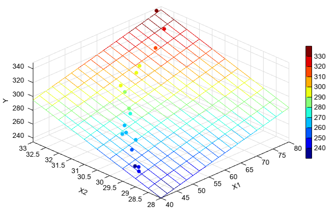
多元线性回归的函数是mlinregress。

y = array([251.3, 251.3, 248.3, 267.5, 273.0, 276.5, 270.3, 274.9, 285.0 \
      , 290.0, 297.0, 302.5, 304.5, 309.3, 321.7, 330.7, 349.0])
x1 = array([41.9,  43.4,  43.9,  44.5,  47.3,  47.5,  47.9,  50.2,  52.8 \
      , 53.2,  56.7,  57.0,  63.5,  65.3,  71.1,  77.0,  77.8])
x2 = array([29.1,  29.3,  29.5,  29.7,  29.9,  30.3,  30.5,  30.7,  30.8 \
      , 30.9,  31.5,  31.7,  31.9,  32.0,  32.1,  32.5,  32.9])
x = zeros((len(y), 2))
x[:,0] = x1
x[:,1] = x2
byta, residuals = np.stats.mlinregress(y, x)
print(byta.astype('float'))
print(residuals.astype('float'))
print('y = %.2f + %.2fx1 + %.2fx2' % \
    (byta[0], byta[1], byta[2]))

#plot
scatter3(x1, x2, y, c=y)
xx, yy = meshgrid(arange(40, 80.1, 2), arange(28, 33.1, 0.5))
z = byta[0] + byta[1] * xx + byta[2] * yy
mesh(xx, yy, z, facecolor=None)
colorbar(shrink=0.8, aspect=30)
xlabel('X1')
ylabel('X2')
zlabel('Y')

卡方检验的适合度和独立性分析函数分别是chisquare和chi2_contingency。

>>> stats.chisquare([16, 18, 16, 14, 12, 12], [16, 16, 16, 16, 16, 8])
(3.5, 0.623387627749582)
>>> obs = array([[10, 10, 20], [20, 20, 20]])
>>> stats.chi2_contingency(obs)
(2.7777777777777777, 0.24935220877729614)

T检验包括三个函数：ttest_1samp用来进行单样本T检验；ttest_ind用来进行两个独立样本T检验；ttest_rel用来进行配对 样本T检验。

>>> a = array([1,2,-1,2,1,-4])
>>> mu = 0
>>> stats.ttest_1samp(a, mu)
(0.17622684421256019, 0.8670310908282268)
>>> x=array([ 0.01082045,0.00225922,0.00022592,0.00011891,0.00525565,0.00156956])
>>> y=array([ 0.0096333,0.0019453,0.0038384,0.0058286,0.00078786])
>>> stats.ttest_ind(x, y)
(-0.45068935600352156, 0.6628942089591048)
>>> a = [3,5,4,6,5,5,4,5,3,6,7,8,7,6,7,8,8,9,9,8,7,7,6,7,8]
>>> b = [7,8,6,7,8,9,6,6,7,8,8,7,9,10,9,9,8,8,4,4,5,6,9,8,12]
>>> stats.ttest_rel(a, b)
(-2.449489742783178, 0.021982997044102233)

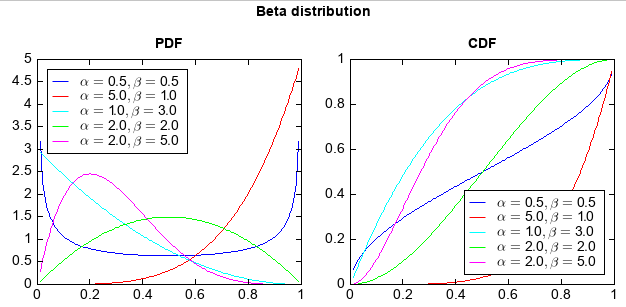
numeric.stats包中还有多种概率分布函数，包括：norm、beta、cauchy、chi2、expon、f、gamma、gumbel、laplace、 levy、logistic、lognorm、nakagami、pareto、t、triang、uniform、weibull。下面给出一个Beta分布的示例，其他 的都类似。

x = arange(0.01, 1, 0.01)
aa = [0.5, 5, 1, 2,2]
bb = [0.5, 1, 3, 2 ,5]
ss = ['-b', '-r', '-c', '-g', '-m']

#PDF
subplot(1,2,1)
for a,b,s in zip(aa,bb,ss):
    y = stats.beta.pdf(x, a, b)
    plot(x, y, s, label=r'$\alpha = %.1f, \beta = %.1f$' % (a, b))
legend(loc='upper left', facecolor='w')
ylim(0, 5)
xlim(0, 1)
title('PDF')

#CDF
subplot(1,2,2)
for a,b,s in zip(aa,bb,ss):
    y = stats.beta.cdf(x, a, b)
    plot(x, y, s, label=r'$\alpha = %.1f, \beta = %.1f$' % (a, b))
legend(loc='lower right', facecolor='w')
ylim(0, 1)
xlim(0, 1)
title('CDF')

suptitle('Beta distribution')