contour3
- mipylib.plotlib.miplot.contour3(*args, **kwargs)
3-D contour plot.
- Parameters:
x – (array_like) Optional. X coordinate array.
y – (array_like) Optional. Y coordinate array.
z – (array_like) 2-D z value array.
levels – (array_like) Optional. A list of floating point numbers indicating the level curves to draw, in increasing order.
cmap – (string) Color map string.
colors – (list) If None (default), the colormap specified by cmap will be used. If a string, like ‘r’ or ‘red’, all levels will be plotted in this color. If a tuple of matplotlib color args (string, float, rgb, etc), different levels will be plotted in different colors in the order specified.
smooth – (boolean) Smooth contour lines or not.
- Returns:
(graphics) Contour graphics created from array data.
Example:
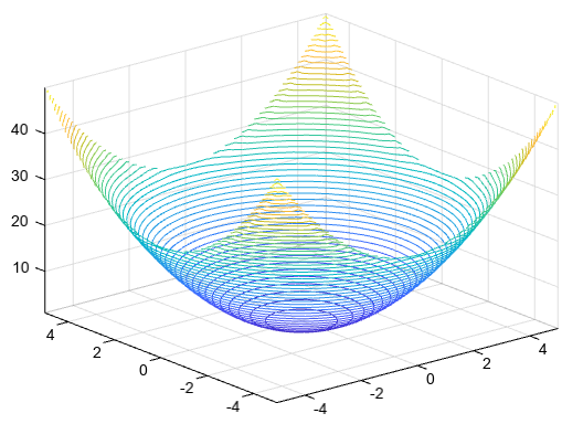
Define Z as a function of two variables, X and Y. Then plot the contours of Z. In this case, let MeteoInfoLab choose the contours and the limits for the x- and y-axes.
[X,Y] = meshgrid(arange(-5,5.2,0.25))
Z = X**2 + Y**2
contour3(X, Y, Z)
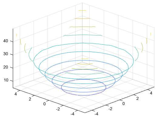
Now specify 50 contour levels, and display the results within the x and y limits used to calculate Z.
[X,Y] = meshgrid(arange(-5,5.2,0.25))
Z = X**2 + Y**2
contour3(X, Y, Z, 50)
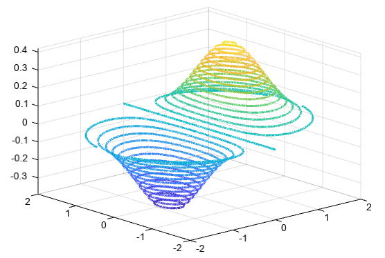
Define Z as a function of two variables, X and Y. Plot 30 contours of Z, and then set the line width to 3.
[X,Y] = meshgrid(arange(-2,2.01,0.0125))
Z = X*exp(-X**2-Y**2)
contour3(X, Y, Z, 30, linewidth=3)