EOF analysis

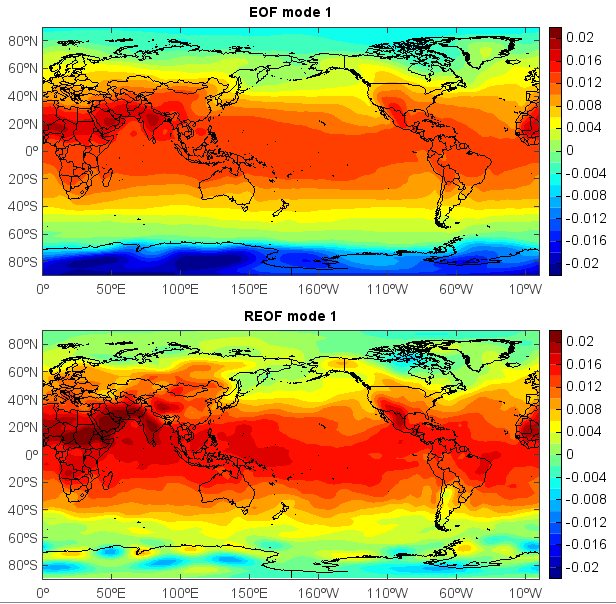
Empirical Orthogonal Function (EOF) analysis is often used to study possible spatial modes (ie, patterns) of variability and how they change with time. In statistics, EOF analysis is known as Principal Component Analysis (PCA). To get localized EOF structures, rotated EOF analysis can be applied. Varimax rotation method is commonly used. The following script does EOF and REOF analysis from a dataset including the 62-year globle temperature of a certain month with dimensions of 71 * 144 * 62.

fn = 'C:/Temp/EOF/test.txt'
ny = 71
nx = 144
m = ny * nx
n = 62
ss1 = asciiread(fn, shape=(71,144,n))
ss1 = ss1[::-1,::1,:]
X = ss1.reshape(ny * nx, n)

#EOF calculation - Time-space transform
EOF, E, PC = meteo.eof(X, transform=True)
eof1 = EOF[:,0].reshape(ny, nx)

#REOF calculation using varimax rotation
REOF = meteo.varimax(EOF[:,:5])[0]
reof1 = REOF[:,0].reshape(ny, nx)

#Plot
lon = linspace(0, 360, nx)
lat = linspace(-90, 90, ny)
#EOF mode 1
subplot(2,1,1)
axesm(newaxes=False)
geoshow('country', edgecolor='k')
levs = arange(-0.02, 0.021, 0.002)
layer = contourf(lon, lat, eof1, levs, smooth=False)
colorbar(layer)
title('EOF mode 1')
#REOF mode 1
subplot(2,1,2)
axesm(newaxes=False)
geoshow('country', edgecolor='k')
levs = arange(-0.02, 0.021, 0.002)
layer = contourf(lon, lat, reof1, levs, smooth=False)
colorbar(layer)
title('REOF mode 1')

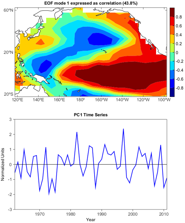
Compute and plot the leading EOF of sea surface temperature in the central and northern Pacific during winter time.

The spatial pattern of this EOF is the canonical El Nino pattern, and the associated time series shows large peaks and troughs for well-known El Nino and La Nina events.

from mipylib.numeric import stats

#Read data
f = addfile('D:/Temp/nc/sst_ndjfm_anom.nc')
sst = f['sst'][:,:,:]
lon = f['longitude'][:]
lat = f['latitude'][:]

#Square-root of cosine of latitude weights are applied before the
#computation of EOFs.
clat = sqrt(cos(radians(lat)))
clat = clat.reshape(1, clat.shape[0], 1)
clat = broadcast_to(clat, sst.shape)
sst = sst * clat

#reorder to (lat * lon, time)
nt, ny, nx = sst.shape
X = sst.reshape(nt, ny * nx)
X = X.T

#EOF calculation
EOF, E, PC = meteo.eof(X, svd=True)
eof1 = EOF[:,0].reshape(ny, nx)
pc1=(PC[0,:] - mean(PC[0,:])) / std(PC[0,:])
e1 = E[0] / sum(E) * 100

#Correlation between PC1 and sst
eof1_cor = ones([ny,nx]) * nan
x = PC[0,:]
for i in arange(ny):
    for j in arange(nx):
        y=sst[:,i,j]
        eof1_cor[i,j] = stats.pearsonr(x, y)[0]

#Plot
subplot(2,1,1)
axesm(newaxes=False)
geoshow('continent', edgecolor='k', facecolor='w')
levs = arange(-0.8, 1, 0.2)
layer = contourf(lon, lat, eof1_cor, levs, smooth=False, order=0)
yticks(arange(-20, 61, 40))
colorbar(layer)
title('EOF mode 1 expressed as correlation (%.1f%%)' % e1)

subplot(2,1,2)
years = range(1962, 2012)
plot(years, pc1,color='b',linewidth=2)
y = zeros(nt)
plot(years, y, color='k')
xlim(1962, 2011)
ylim(-3,3)
xticks(arange(1970,2011,10))
xaxis(tickin=False)
xaxis(tickvisible=False, location='top')
yaxis(tickin=False)
yaxis(tickvisible=False, location='right')
xlabel('Year')
ylabel('Normalized Units')
title('PC1 Time Series')