Frontogenesis Analysis

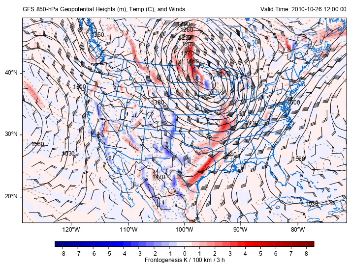
Frontogenesis at 850-hPa with Geopotential Heights, Temperature, and Winds

This example uses example data from the GFS analysis for 12 UTC 26 October 2010 and calculates frontogenesis and wind speed with geographic plotting.

fn = 'D:/Temp/nc/GFS_20101026_1200.nc'
f = addfile(fn)

# Set subset slice for the geographic extent of data
lon_slice = slice(400, 650)
lat_slice = slice(50, 150, -1)

# Grab lat/lon values (GFS will be 1D)
lats = f['lat'][lat_slice]
lons = f['lon'][lon_slice]

level = '85000'
hght_850 = f['Geopotential_height_isobaric'][0, level, lat_slice, lon_slice]
tmpk_850 = f['Temperature_isobaric'][0, level, lat_slice, lon_slice]
uwnd_850 = f['u-component_of_wind_isobaric'][0, level, lat_slice, lon_slice]
vwnd_850 = f['v-component_of_wind_isobaric'][0, level, lat_slice, lon_slice]

# Convert temperatures to degree Celsius for plotting purposes
tmpc_850 = tmpk_850 - 273.15

# Calculate potential temperature for frontogenesis calculation
thta_850 = meteolib.potential_temperature(850, tmpk_850)

dx, dy = meteolib.lat_lon_grid_deltas(lons, lats)
fronto_850 = meteolib.frontogenesis(thta_850, uwnd_850, vwnd_850, dx, dy)

# A conversion factor to get frontogensis units of K per 100 km per 3 h
convert_to_per_100km_3h = 1000*100*3600*3

#plot
proj = projinfo(proj='lcc', lon_0=-100, lat_0=35, lat_1=30, lat_2=60)
ax = axesm(projinfo=proj, tickfontsize=12)
geoshow('us_states', edgecolor=(0,102,204))
geoshow('country', edgecolor=(0,102,204))

# Plot 850-hPa Frontogenesis
clevs_fronto = np.arange(-8, 8.5, 0.5)
cf = contourf(lons, lats, fronto_850*convert_to_per_100km_3h, clevs_fronto,
                 cmap='BlWhRe', smooth=False)
colorbar(cf, orientation='horizontal', shrink=0.8, aspect=50, fontsize=12,
    label='Frontogenesis K / 100 km / 3 h')

# Plot 850-hPa Temperature in Celsius
clevs_tmpc = np.arange(-40, 41, 2)
csf = contour(lons, lats, tmpc_850, clevs_tmpc, colors='gray',
                 linestyle='--')
clabel(csf, fmt='%d', fontsize=12, drawshadow=False)

# Plot 850-hPa Geopotential Heights
clevs_850_hght = np.arange(0, 8000, 30)
cs = contour(lons, lats, hght_850, clevs_850_hght, colors='black')
clabel(cs, fmt='%d', fontsize=12, drawshadow=False)

# Plot 850-hPa Wind Barbs only plotting every fifth barb
wind_slice = (slice(None, None, 5), slice(None, None, 5))
barbs(lons[wind_slice[0]], lats[wind_slice[1]],
         uwnd_850[wind_slice], vwnd_850[wind_slice],
         color='black')

axis([-128, -72, 16, 55])

# Plot some titles to tell people what is on the map
left_title(r'GFS 850-hPa Geopotential Heights (m), Temp (C), and Winds', fontsize=12, bold=False)
right_title('Valid Time: {}'.format(f.gettime(0)), fontsize=12, bold=False)