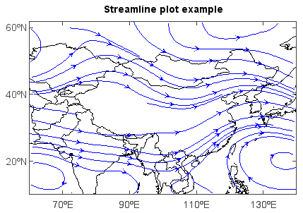
Streamline plot

Streamline plot was created by streamplot() function.

fn = os.path.join(migl.get_sample_folder(), 'GrADS', 'model.ctl')
f = addfile(fn)
u = f['U'][0,'500','10:60','60:140']
v = f['V'][0,'500','10:60','60:140']

#Plot
axesm()
geoshow('country', edgecolor='k')
layer = streamplotm(u, v)
title('Streamline plot example')
yticks([20,40,60])

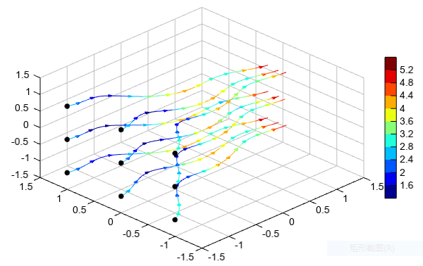
3D streamline plot was created by streamplot3() function.

# Make the grid
x, y, z = meshgrid(arange(-1.5, 1.5, 0.1),
                   arange(-1.5, 1.5, 0.1),
                   arange(-1.5, 1.5, 0.1))

# Make the direction data for the arrows
u = x + cos(4*x) + 3         # x-component of vector field
v = sin(4*x) - sin(2*y)      # y-component of vector field
w = -z                       # z-component of vector field
speed = sqrt(u*u + v*v + w*w)

sx, sy, sz = meshgrid([-1.5], [-1,0,1], [-1,0,1])

qq = streamplot3(x[0,0,:], y[0,:,0], z[:,0,0], u, v, w, speed, linewidth=1,
    density=4, interval=10, start_x=sx, start_y=sy, start_z=sz)
scatter3(sx, sy, sz, c='k')
colorbar(qq)
xlim(-1.5, 1.5)
ylim(-1.5, 1.5)
zlim(-1.5, 1.5)

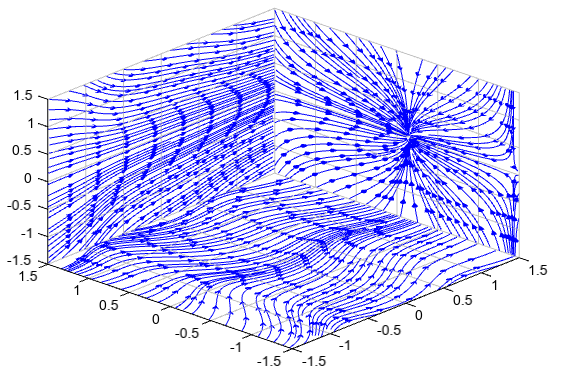
Plot streamlines in slice planes.

# Make the grid
x, y, z = meshgrid(arange(-1.5, 1.6, 0.1),
                   arange(-1.5, 1.6, 0.1),
                   arange(-1.5, 1.6, 0.1))

# Make the direction data for the arrows
u = x + cos(4*x) + 3         # x-component of vector field
v = sin(4*x) - sin(2*y)      # y-component of vector field
w = -z                       # z-component of vector field
speed = sqrt(u*u + v*v + w*w)

streamslice(x, y, z, u, v, w, xslice=1.5, yslice=1.5, zslice=-1.5,
    color='b', linewidth=1, density=4, interval=5)
xlim(-1.5, 1.5)
ylim(-1.5, 1.5)
zlim(-1.5, 1.5)