Windrose plot
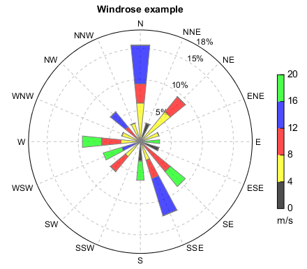
Windrose can be plotted using windrose function with wind direction and wind speed data.
fn = r'D:\Temp\ascii\windrose.txt'
ncol = numasciicol(fn)
nrow = numasciirow(fn)
a = asciiread(fn,shape=(nrow,ncol))
ws=a[:,0]
wd=a[:,1]

n = 16
wsbins = arange(0., 21.1, 4)
cols = makecolors(['k','y','r','b','g'], alpha=0.7)
rtickloc = [0.05,0.1,0.15,0.18]
ax, bars = windrose(wd, ws, n, wsbins, rmax=0.18, colors=cols, rtickloc=rtickloc)
colorbar(bars, shrink=0.6, vmintick=True, vmaxtick=True, xshift=10, \
    label='m/s', labelloc='bottom')
title('Windrose example')
In fact, windrose is plotted in a polar axes. But there are some diffenrence between windrose
and polar coordinates. The polar angle theta is the counterclockwise angle from the x-axis in
polar coordinates, meanwhile the polar angle theta is the clockwise angle from the y-axis in
windrose coordinates. So the wind direction data have to be converted from windrose coordinates
to polar coordinates for visualization purpose. The conversion processe was done in windorose
function. Also you can do it in the code to plot windrose without windrose function.
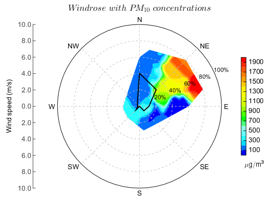
The below example will plot PM10 concentration with filled contours and wind direction frequency. The following data were used.
WS WD PM10
1 335 183.2
4 350 173.4
2 0 194
1 0 175.75
3 0 203.6
3 0 161.2
3 0 142
2 0 163
2 0 175.5
1 0 208.4
1 0 205
1 0 171.2
3 170 143.6
3 135 116
3 135 110.6
2 135 93.2
5 90 98.2
4 90 91.8
6 90 83.6
4 90 88.4
2 100 81.4
1 80 77
2 0 81.8
3 0 89.4
3 0 115.8
3 0 131.2
4 0 166.4
3 0 174
3 0 170.2
7 10 152.4
6 0 184.4
7 20 203.8
4 30 212.6
8 45 627.8
6 45 1290.4
6 45 1581.25
7 80 1711.525
7 45 1841.8
6 45 2128.4
8 75 2406.8
8 45 2576.8
8 45 2035.6
7 45 1615
5 60 1286.8
4 45 1202.4
3 70 1015.2
3 80 733.8
1 90 635.6
2 225 339.2
2 270 331.4
2 260 303.2
2 225 282.6
The PM10 data was plotted in a Cartesian axes and the wind direction frequency line was plotted in a polar axes. The two axes must have same position.
def windrose2polar(a):
    """
    Convert wind direction towindrose polar coordinate
    """
    r = 360 - a + 90
    r[r>360] = r - 360
    return r

#Read data (wind speed, weed direction, pm10)
fn = os.path.join(migl.get_sample_folder(), 'ASCII', 'pm10.txt')
df = DataFrame.read_table(fn, format='%3f')
ws = df['WS'].values
wd = df['WD'].values
pm10 = df['PM10'].values
N = len(ws)

#Convert from windrose coordinate to polar coordinate
rwd = windrose2polar(wd)

#Degree to radians
rwd = radians(rwd)

#Calculate frequency of each wind direction bin
wdbins = linspace(0.0, pi * 2, 9)
dwdbins = degrees(wdbins)
dwdbins = windrose2polar(dwdbins)
rwdbins = radians(dwdbins)
wdN = len(wdbins) - 1
theta = ones(wdN + 1)
for j in range(wdN):
    theta[j] = rwdbins[j]
theta[wdN] = theta[0]
wd = wd + 360./wdN/2
wd[wd>360] = wd - 360
wdhist = histogram(radians(wd), wdbins)[0].astype('float')
wdhist = wdhist / N
nwdhist = wdhist.aslist()
nwdhist.append(nwdhist[0])
nwdhist = array(nwdhist)

#Polar coordinate to Cartesian coordinate
rwdc, wsc = pol2cart(rwd, ws)

#Get convexhull (minimum outer polygon of the wind points)
poly = topo.convexhull(rwdc, wsc)

#Get grid data
dd = 0.5
x = linspace(rwdc.min() - dd, rwdc.max() + dd, 50)
y = linspace(wsc.min() - dd, wsc.max() + dd, 50)
data = griddata((rwdc, wsc), pm10, xi=(x, y), method='idw', pointnum=5, convexhull=False)[0]

#---------------------------------------
#Plot figure
pos = [0.13, 0.1, 0.775, 0.775]

#Cartesian axes
ax = axes(position=pos, aspect='equal')
xaxis(visible=False)
yaxis(location='right', visible=False)
yaxis(location='left', shift = 50)
ylabel('Wind speed (m/s)')
levs = arange(100, 2000, 100)
cg = contourf(x, y, data, levs, edgecolor=None, cmap='BlAqGrYeOrRe', visible=False)
cg = cg.clip([poly])
ax.add_graphic(cg)
colorbar(cg, shrink=0.6, xshift=30, label=r'$\mu g/m^3$', labelloc='bottom')
maxv = 10
xlim(-maxv, maxv)
ylim(-maxv, maxv)
ticks = ax.get_yticks()
ax.set_yticklabels([abs(yy) for yy in ticks])

#Polar axes
axp = axes(position=pos, polar=True)
plot(theta, nwdhist, color='k', linewidth=2)
axp.set_rmax(1)
axp.set_rlabel_position(25.)
axp.set_rtick_locations([0.2,0.4,0.6,0.8,1])
axp.set_rticks(['20%','40%','60%','80%','100%'])
axp.set_xtick_font(size=14)
axp.set_xticks(['E','NE','N','NW','W','SW','S','SE'])
title(r'$Windrose \ with \ PM_{10} \ concentrations$', fontsize=18)
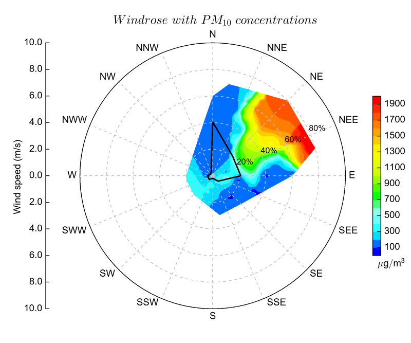
PM10 windrose plot with 16 direction labels:
def windrose2polar(a):
    r = 360 - a + 90
    r[r>360] = r - 360
    return r

#Read data (wind speed, weed direction, pm10)
fn = r'D:\Temp\ascii\pm10.txt'
table = readtable(fn, format='%3f')
ws = table['WS']
wd = table['WD']
pm10 = table['PM10']
N = len(ws)

#Convert from windrose coordinate to polar coordinate
rwd = windrose2polar(wd)

#Degree to radians
rwd = radians(rwd)

#Calculate frequency of each wind direction bin
wdbins = linspace(0.0, pi * 2, 9)
dwdbins = degrees(wdbins)
dwdbins = windrose2polar(dwdbins)
rwdbins = radians(dwdbins)
wdN = len(wdbins) - 1
theta = ones(wdN + 1)
for j in range(wdN):
    theta[j] = rwdbins[j]
theta[wdN] = theta[0]
wd = wd + 360./wdN/2
wd[wd>360] = wd - 360
wdhist = histogram(radians(wd), wdbins)[0].astype('float')
wdhist = wdhist / N
nwdhist = wdhist.aslist()
nwdhist.append(nwdhist[0])
nwdhist = array(nwdhist)

#Polar coordinate to Cartesian coordinate
rwdc, wsc = pol2cart(rwd, ws)

#Get convexhull (minimum outer polygon of the wind points)
poly = topo.convexhull(rwdc, wsc)

#Get grid data
dd = 0.5
x = linspace(rwdc.min() - dd, rwdc.max() + dd, 50)
y = linspace(wsc.min() - dd, wsc.max() + dd, 50)
data = griddata((rwdc, wsc), pm10, xi=(x, y), method='idw', pointnum=5, convexhull=False)[0]

#---------------------------------------
#Plot figure
pos = [0.13, 0.1, 0.775, 0.775]

#Cartesian axes
ax = axes(position=pos, aspect='equal')
xaxis(visible=False)
yaxis(location='right', visible=False)
yaxis(location='left', shift = 50)
ylabel('Wind speed (m/s)')
levs = arange(100, 2000, 100)
cg = contourf(x, y, data, levs, cmap='BlAqGrYeOrRe', visible=False)
cg = cg.clip([poly])
ax.add_graphic(cg)
#ss = scatter(rwdc, wsc, s=6, fill=False, edgecolor='b', edgesize=1)
#patch(poly)
colorbar(cg, shrink=0.6, xshift=30, label=r'$\mu g/m^3$', labelloc='bottom')
maxv = 10
xlim(-maxv, maxv)
ylim(-maxv, maxv)
ticks = ax.get_yticks()
ax.set_yticklabels([abs(yy) for yy in ticks])

#Polar axes
axp = axes(position=pos, polar=True)
plot(theta, nwdhist, color='k', linewidth=2)
axp.set_rmax(1)
axp.set_rlabel_position(25.)
axp.set_rtick_locations([0.2,0.4,0.6,0.8])
#axp.set_rticks(['2','4','6','8','10 m/s'])
axp.set_rticks(['20%','40%','60%','80%'])
axp.set_xtick_font(size=14)
axp.set_xtick_locations(arange(0,360,22.5))
axp.set_xticks(['E','NEE','NE','NNE','N','NNW','NW','NWW','W','SWW',
    'SW','SSW','S','SSE','SE','SEE'])
title(r'$Windrose \ with \ PM_{10} \ concentrations$', fontsize=18)
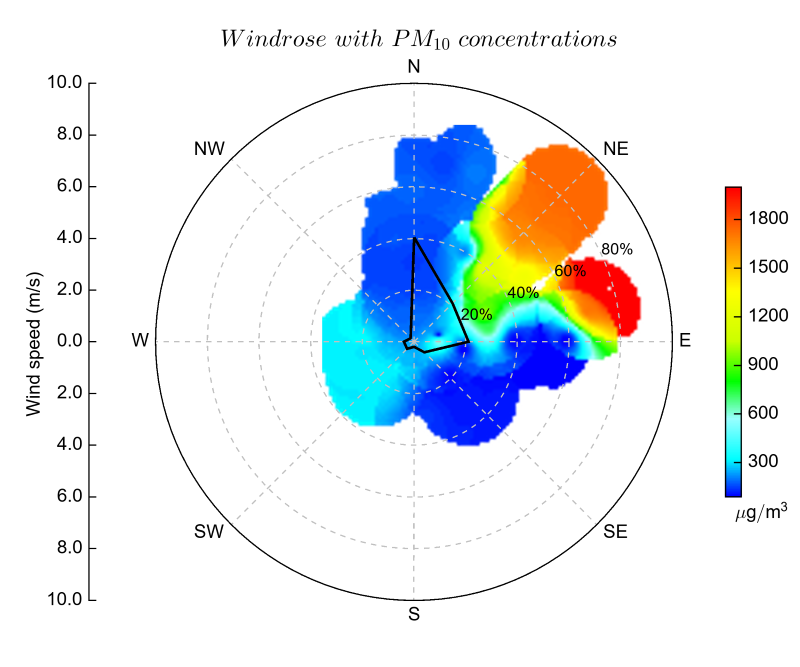
Plot PM10 data with imshow function:
def windrose2polar(a):
    r = 360 - a + 90
    r[r>360] = r - 360
    return r

#Read data (wind speed, weed direction, pm10)
fn = r'D:\Temp\ascii\pm10.txt'
table = readtable(fn, format='%3f')
ws = table['WS']
wd = table['WD']
pm10 = table['PM10']
N = len(ws)

#Convert from windrose coordinate to polar coordinate
rwd = windrose2polar(wd)

#Degree to radians
rwd = radians(rwd)

#Calculate frequency of each wind direction bin
wdbins = linspace(0.0, pi * 2, 9)
dwdbins = degrees(wdbins)
dwdbins = windrose2polar(dwdbins)
rwdbins = radians(dwdbins)
wdN = len(wdbins) - 1
theta = ones(wdN + 1)
for i in range(wdN):
    #theta[i] = rwdbins[i] - pi/wdN
    theta[i] = rwdbins[i]
theta[wdN] = theta[0]
wd = wd + 360./wdN/2
wd[wd>360] = wd - 360
wdhist = histogram(radians(wd), wdbins)[0].astype('float')
wdhist = wdhist / N
nwdhist = wdhist.aslist()
nwdhist.append(nwdhist[0])
nwdhist = array(nwdhist)

#Polar coordinate to Cartesian coordinate
rwdc, wsc = pol2cart(rwd, ws)

#Get convexhull (minimum outer polygon of the wind points)
poly = topo.convexhull(rwdc, wsc)

#Get grid data
dd = 1.5
x = linspace(rwdc.min() - dd, rwdc.max() + dd, 100)
y = linspace(wsc.min() - dd, wsc.max() + dd, 100)
data = griddata((rwdc, wsc), pm10, xi=(x, y), method='idw', radius=2)[0]

#---------------------------------------
#Plot figure
pos = [0.13, 0.1, 0.775, 0.775]

#Cartesian axes
ax = axes(position=pos, aspect='equal')
xaxis(visible=False)
yaxis(location='right', visible=False)
yaxis(location='left', shift = 50)
ylabel('Wind speed (m/s)')
levs = arange(100, 2000, 10)
cg = imshow(data, levs, cmap='BlAqGrYeOrRe', extent=[x[0],x[-1],y[0],y[-1]], \
    interpolation='bicubic')
colorbar(cg, ticks=arange(0, 2001, 300), shrink=0.6, xshift=30, label=r'$\mu g/m^3$', labelloc='bottom')
maxv = 10
xlim(-maxv, maxv)
ylim(-maxv, maxv)
ticks = ax.get_yticks()
ax.set_yticklabels([abs(yy) for yy in ticks])

#Polar axes
axp = axes(position=pos, polar=True)
plot(theta, nwdhist, color='k', linewidth=2)
axp.set_rmax(1)
axp.set_rlabel_position(25.)
axp.set_rtick_locations([0.2,0.4,0.6,0.8,1])
axp.set_rticks(['20%','40%','60%','80%','100%'])
axp.set_xtick_font(size=14)
axp.set_xticks(['E','NE','N','NW','W','SW','S','SE'])
title(r'$Windrose \ with \ PM_{10} \ concentrations$', fontsize=18)