FY-4A AGRI data

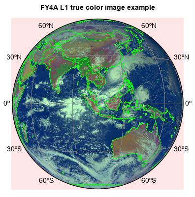
This example code illustrates how to access and visualize a FY-4A L1 satellite data. Channel 1 (470nm), channel 2 (650nm) and channel 3 (830nm) data are used to composite a true color image.

fn = 'D:/Temp/LaSW/airship/FY4A/FY4A-_AGRI--_N_DISK_1047E_L1-_FDI-_MULT_NOM_20221031060000_20221031061459_4000M_V0001.HDF'
f = addfile(fn)

B = f['NOMChannel01'][::-1]
G = f['NOMChannel02'][::-1]
R = f['NOMChannel03'][::-1]
B = B / 4095.
G = G / 4095.
R = R / 4095.
B[B>1] = nan
G[G>1] = nan
R[R>1] = nan
R_G = R / G
R = R * 0.8
R1 = R.copy()

C = R_G > 2
R[C] = G
G[C] = R1

x = linspace(-5496000.0,5496000.0, 2748)
y = linspace(-5496000.0,5496000.0, 2748)

#Plot
proj = projinfo(proj='geos', lon_0=104.7, height=35786000.0)
figure()
axesm(projection=proj, gridlabelloc='all', griddx=30,
    griddy=30, gridline=True, frameon=False)
geoshow('country', edgecolor='g')
layer = imshow(x, y, [R,G,B], interpolation='bilinear', proj=proj)
#Adjust image
imagelib.hsb_adjust(layer, h=0, s=0.1, b=0.3)
title('FY4A L1 true color image example')

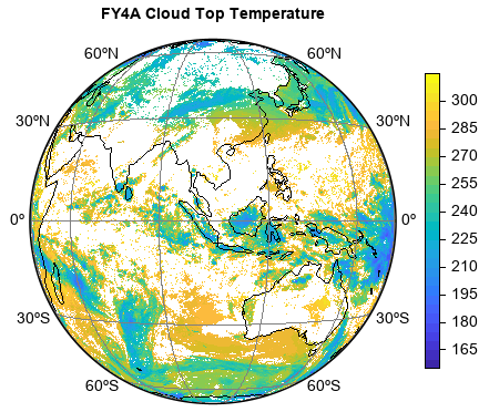
The example to read and plot FY4A l2 CTT data.

fn = 'D:/Temp/FY/FY4A-_AGRI--_N_DISK_1047E_L2-_CTT-_MULT_NOM_20190209140000_20190209141459_4000M_V0001.NC'
f = addfile(fn)
x = linspace(-5496000.0,5496000.0, 2748)
y = linspace(-5496000.0,5496000.0, 2748)
data = f['CTT'][::-1,:]
data[data>1000] = nan
data[data==-999] = nan
height = f['nominal_satellite_height'][:]

#Plot
lon0 = 104.7
ax = axesm(proj='geos', lon_0=lon0, h=height, gridlabelloc='all', griddx=30,
    griddy=30, gridline=True, frameon=False)
geoshow('coastline', color='k')
levs = arange(160, 311, 5)
layer = imshow(x, y, data, levs, proj=ax.proj)
colorbar(layer, shrink=0.8, xshift=15)
title('FY4A Cloud Top Temperature')